- - Clarify Any Formula - -
PrecisionCalc
- - Clarify Any Formula
- -
Tutorial
To install The Formulator, simply download the file, double-click on it, and follow the instructions. Then, if Excel was running, exit and restart Excel.
Important:
On Windows NT, 2000, XP, Vista, 7, 8, 8.1, and 10, you must be logged in as an Administrator
during installation. On Windows Vista, 7, 8, 8.1, and
10, start Setup by
right-clicking TheFormulator.exe and choosing "Run as administrator":

After installation, you no longer need to be logged in as an Administrator.
After installing The Formulator, start Excel (or restart Excel if it was already running).
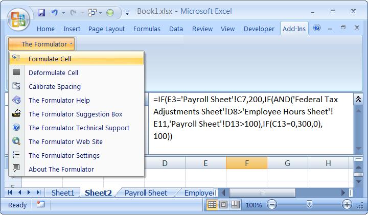
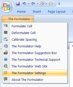
After installing the Formulator, find its menu in Excel by choosing Add-Ins > The Formulator:
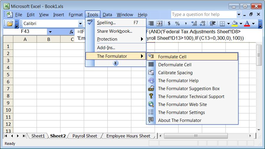
In Excel 2003 and earlier, The Formulator's menu is in Tools > The Formulator:
Enter this simple formula in Excel:
=IF(A1>B1,100,200)
With that cell selected, select The Formulator | Formulate Cell.
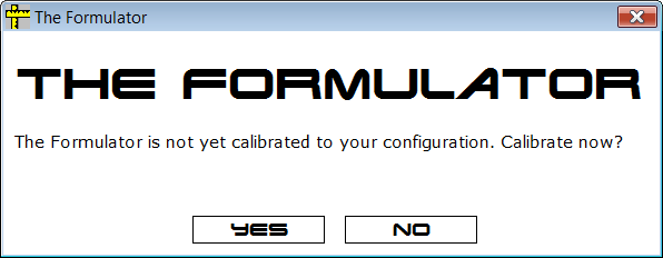
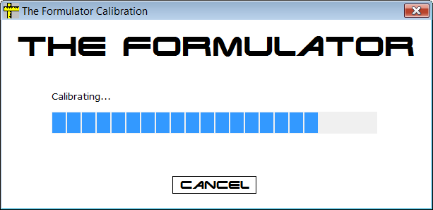
If this is the first time you have formatted a formula with The Formulator on this computer, it will prompt you to calibrate. Calibration is required for The Formulator to correctly format formulas:
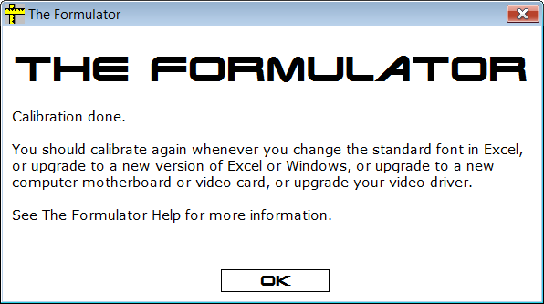
After calibration is complete, The Formulator indents the three arguments and lines up the two parens, like this:
=IF(
A1>B1,
100,
200
)
Note that the formula correctly returns 200. If you enter 1 in cell A1, the formula correctly returns 100. The formatting inserted by The Formulator has absolutely no effect on the results returned by the formula.
Select The Formulator | Deformulate Cell. The Formulator removes the formatting.
Change the name of one of the other sheets to "Sheet Name" (with a space). Then, go back to the sheet with the formula, and change the formula to this, making sure to include the spaces in "a b c":
=IF(A1>B1,100,IF('Sheet Name'!A1="a b c",200,300))
With that cell selected, select The Formulator | Formulate Cell. The Formulator indents the second IF function to the position of the arguments of the first IF function, and it indents the second IF functions three arguments and lines up its parens:
=IF(
A1>B1,
100,
IF(
'Sheet Name'!A1="a b c",
200,
300
)
)
Note that you can easily identify any function's arguments and parens by looking up and down, because they are lined up vertically.
While the formula is still formatted, change it to this:
=IF(
A1>B1,
100,
IF(
'Sheet Name'!A1="a b c",
200,
400
)
)
Note that the value returned by the formula changes from 300 to 400. You can make any edits to any formula formatted by The Formulator that you could make on the same non-formatted formula.
Select The Formulator | Deformulate Cell. Note that when The Formulator removes the formatting, it preserves the spaces in "Sheet Name" and "a b c".
Change the formula to this, and select The Formulator | Formulate Cell:
=IF(A1>B1,IF('Sheet Name'!A1="a b c",IF(OR(C1>D1,E1<F1),300,400),500),600)
Note that even though some arguments are now widely separated from their siblings, you can still easily identify any function's arguments by looking up and down, because they are lined up vertically.
=IF(
A1>B1,
IF(
'Sheet Name'!A1="a b c",
IF(
OR(
C1>D1,
E1<F1
),
300,
400
),
500
),
600
)
The Formulator recognizes, and leaves unformatted, string literal parens. Enter this formula, and select The Formulator | Formulate Cell:
=IF(A1="James Cameron (Director)",100,200)
Result: The Formulator recognizes the parens around "Director" to be string literals, and does not format them:
=IF(
A1="James Cameron (Director)",
100,
200
)
If your formula has parens right after arithmetic operators, you might prefer that they not be formatted. Enter this formula, and select The Formulator | Formulate Cell:
=IF(A1>B1,100,200)+(C1-D1)/E1
Result: The Formulator formats all parens:
=IF(
A1>B1,
100,
200
)
+(
C1-D1
)
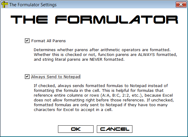
/E1You might prefer to leave the parens after the arithmetic operator unformatted:
=IF(
A1>B1,
100,
200
)
+(C1-D1)/E1To do that, choose The Formulator | The Formulator Settings, and turn off Format All Parens:
You might wonder about some of the formatting choices made by The Formulator. Some of them are due to working around formatting limitations imposed by Excel:
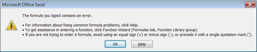
- Carriage returns and spaces between function names and their opening parens are not accepted by Excel (error message pops up).
Try entering this formula:
=IF
(
A1>B1,
100,
200
)Result: Excel displays an error message. Excel does not accept any formatting characters between a function name and its opening paren:
- Carriage returns and spaces right before commas are silently removed by Excel (no error message).
Try entering this formula:
=IF(
A1>B1
,
100
,
200
)Result: Excel silently (no error message) changes the formula to this. Excel does not accept any formatting characters right before commas:
=IF(
A1>B1,
100,
200
)
- Carriage returns and spaces before an entire-column or entire-row reference (such as A:A, B:C, 2:2, etc.) are silently removed by Excel (no error message).
Try entering this formula:
=SUM(
A:A
)Result: Excel silently (no error message) changes the formula to this. Excel does not accept any formatting characters right before entire-column or entire-row references:
=SUM(A:A
)Oddly, in addition to removing the formatting characters right before the entire-column or entire-row reference, Excel also inserts a carriage return after the entire-column or entire-row reference.
If your formula is adversely affected by this Excel limitation when formatting it with The Formulator, you might want to set The Formulator to always send the results to Notepad instead of formatting in the cell:
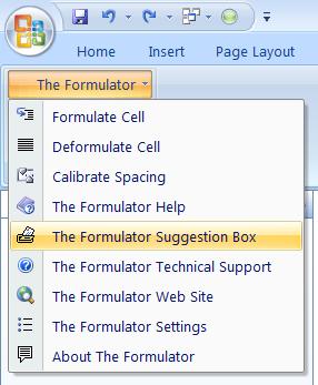
You'll probably soon have ideas about more formatting options and other features you want The Formulator to offer. I want to hear your ideas! Please use the "The Formulator Suggestions Box" from The Formulator menu to send your ideas, suggestions, complaints, etc.:
The
Formulator
Home Page
PrecisionCalc Home Page