PrecisionCalc
inspector
text
Do Anything with Text in Formulas
Tutorial
To install inspector text, simply download the file, double-click on it, and follow the instructions. Then, if Excel was running, exit and restart Excel.
Important:
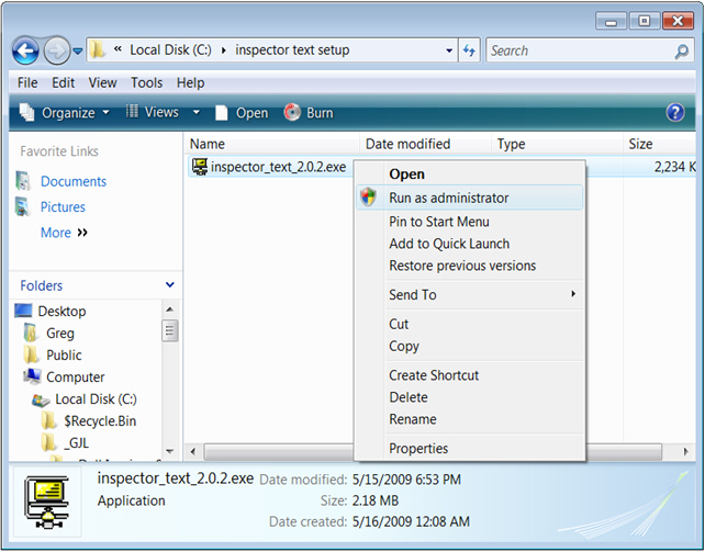
On Windows NT, 2000, XP and Vista, you must be logged in as an Administrator
during installation. On Windows Vista, start Setup by
right-clicking
inspector_text_2.0.2.exe and choosing "Run as administrator":
After installation, you no longer need to be logged in as an Administrator.
After installing inspector text, start Excel (or restart Excel if it was already running).
To verify that inspector text is installed and working properly, enter this formula in any spreadsheet cell:
=itTEST()
It should return a welcome message with your name and the inspector text version. If it instead returns "#NAME!", then inspector text is not correctly installed. You may wish to try installing again, or see the Troubleshooting FAQ, or email for help.
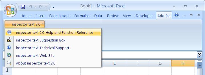
Find inspector text's online help by choosing Add-Ins > inspector text 2.0 > inspector text 2.0 Help and Function Reference:
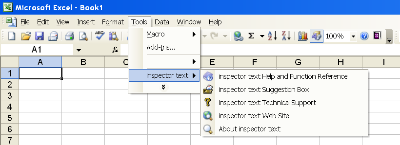
In Excel 2003 and earlier, inspector text's online help is in choosing Tools > inspector text 2.0 > inspector text 2.0 Help and Function Reference:
Search & Replace Functions
inspector text's search and replace functions include itSEARCH, itREPLACE, itCOUNTINCELL, itGETWORD, itEXCLUDE, itEXCLUDENOTNUM, itEXTRACT, itEXTRACTNUM, and itREGEX.
itSEARCH
Allows extremely versatile and flexible text searching. But to get started, try a very simple search formula that although you could do just as well in Excel, will get you acquainted with inspector text:
In cell A1, enter:
abcde
In cell B1, enter this formula:
=itSEARCH(A1,"b")
It returns:
2
That's the position number from the left where b was found.
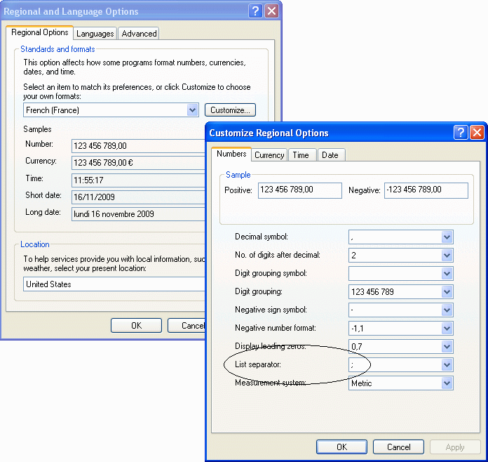
Depending on your world region and language, you might need to use a different character than the comma. Use whatever character you normally use to separate arguments in Excel functions. In many locales, that character is a semi-colon (;). If you're not sure, go into Windows' Regional/Language Options Control Panel and find your "List Separator" character. Use that character wherever inspector text documentation shows a comma. This example shows that the list separator character for French is the semi-colon:
Suppose you don't know, and don't care, whether the B is upper case or lower case. Change cell A1 to this:
aBcDe
And, change the formula in A2 to this:
=itSEARCH(A1,"b",FALSE)
It still returns 2, even though the case doesn't match. The 3rd argument is case_sensitive, and setting it to FALSE makes the formula not case sensitive.
Suppose you're looking for not just the b, but everything from the b through the d, inclusive. Change the formula to this:
=itSEARCH(A1,"b*d",FALSE)
It still returns 2, because that's still the position where the matched string was found.
Suppose you want to know exactly what string it found. Change the formula to this:
=itSEARCH(A1,"b*d",FALSE,3)
It returns the string it found:
BcD
The fourth argument is return_type. itSEARCH offers 22 return types. Here are more examples of different return types:
Suppose you want to know the length of the string it found. Change the formula to this:
=itSEARCH(A1,"b*d",FALSE,4)
It returns the length of "BcD":
3
Suppose you only cared whether or not it found a string that matched the criteria. Change the formula to this:
=itSEARCH(A1,"b*d",FALSE,21)
It returns TRUE, because it found the string for which it searched.
Suppose there might be more than one match, and you want all the matches. Change cell A1 to this:
aBcDebwwDxyz123Bdx00zbd00zx
And, array-enter the following formula in cells A4:A7:
=itSEARCH(A1,"b*d",FALSE,13)
If you're not sure how to array-enter the formula, here's how:
- Select cells A4:A7.
- With all of those cells selected, paste the formula in cell A3. Do not press Enter yet!
- With all of those cells still selected, and with cell A3 still in Edit Mode (because you haven't pressed Enter yet), press and hold down the CTRL and SHIFT keys.
- With all of those cells still selected, and with the CTRL and SHIFT keys still held down, press Enter.
You should see the following results in those four cells:
- A4: BcD
- A5: bwwD
- A6: Bd
- A7: bd
For details on all 22 return types, see the return_type section of the itSEARCH function reference. Also see the return_type section in the examples at the bottom.
Suppose you want the results arranged in a horizontal array instead of a a vertical array. Array-enter the same formula in cells A10:D10:
=itSEARCH(A1,"b*d",FALSE,13)
You should see the same results in those four horizontal cells:
- A10: BcD
- B10: bwwD
- C10: Bd
- D10: bd
Suppose you want to find not only every instance of b*d, but also every instance of x*z. Array-enter the following formula in cells B4:B9:
=itSEARCH(A1,"(b*d|x*z)",FALSE,13)
You should see the following results:
- B4: BcD
- B5: bwwD
- B6: xyz
- B7: Bd
- B8: x00z
- B9: bd
Suppose you want to find the positions of any of a range of characters or digits, such as e - x, or 2 - 4. Change the formula in B4:B9 to this. You'll need to array-enter it again:
=itSEARCH(A1,"[e-x]",FALSE,11)
You should see the following results:
- B4: 5
- B5: 7
- B6: 8
- B7: 10
- B8: 18
- B9: 27
Suppose you wanted to find a character or string repeated within a certain range of repetitions. Change cell A1 to this:
a1ba2ba3ba4ba5b
And change the formula in cell A2 to this:
=itSEARCH(A1,"(a*b){2,4}",FALSE,3)
The {2,4} means to repeat a*b a minimum of 2 times, and a maximum of 4 times.
It returns a1ba2ba3ba4b, because it stopped after the 4th repetition.
Suppose you wanted to find any character OTHER THAN a given character or set of characters. Array-enter this formula in cells C4:C5:
=itSEARCH(A1,"a[^2-4]b",FALSE,13)
This formula looks for an a, followed by any character other than 2, 3, or 4, followed by b.
You should see the following results:
- C4: a1b
- C5: a5b
For details on all the wildcards and substitutions you can use, see the find_text section of the itSEARCH function reference. Also see the find_text section in the examples at the bottom.
Certain characters have special meaning in itSEARCH, and therefore must be given special treatment to search for them as literal characters. These characters are:
[ \ | ? * ( )
To search for any of these characters, precede them with a backslash. For example, to search for a question mark, use \?. To search for a backslash, use two backslashes. Change cell A1 to this:
ab?cd\ef*gh??ij\\kl**mn
And array-enter this formula into cells D4:D6:
=itSEARCH(A1,"(\?\?|\\\\|\*\*)",FALSE,11)
This formula looks for two question marks in a row, or two backslashes in a row, or two asterisks in a row, and returns an array of their starting positions.
You should see the following results:
- D4: 12
- D5: 16
- D6: 20
Suppose you want to restrict the search to characters to the left of certain other characters. Change cell A1 to this:
bxbb
And enter the following formula in cell A2:
=itSEARCH(A1,"b",FALSE,9,"*x")
This formula returns a count of how many times b occurs somewhere to the left of an x. Without the asterisk before the x, it would only look for x immediately after b, with no other characters between them.
It returns 1, not 3, because the 2nd and 3rd b do not occur before an x.
The 5th argument is find_before_text. find_before_text can use all the same wildcards and substitutions as find_text.
Suppose you want to restrict the search to characters that are NOT to the left of certain other characters. Change the formula in cell A2 to this:
=itSEARCH(A1,"b",FALSE,9,,"*x")
This formula returns a count of how many times b occurs without being somewhere to the left of an x. Without the asterisk before the x, it would only look for x immediately after b, with no other characters between them.
It returns 2, because the 2nd and 3rd b are NOT somewhere to the left of an x.
The 6th argument is find_not_before_text. find_not_before_text can use all the same wildcards and substitutions as find_text.
For details on all restricting searches to text that does or does not occur to the left of other text, see the find_before_text and find_not_before_text sections of the itSEARCH function reference. Also see the find_before_text and find_not_before_text sections in the examples at the bottom.
Suppose you want to search from the right instead of from the left. For example, suppose you wanted to find the last backslash in a computer file path. Change cell A1 to this:
C:\My Files\Misc\January\Final\Sales.xls
And change the formula in cell A2 to this:
=itSEARCH(A1,"\\",,,,,,,TRUE)
This formula looks for the first backslash, but searches from right to left.
It returns the position number, counting from the right, at which it found the backslash:
10
But suppose what you really want is Sales.xls, not the position number of the backslash. Change the formula in cell A2 to this:
=itSEARCH(A1,"\\",,5,,,,,TRUE)
This formula looks for the first backslash, searching from right to left, but instead of returning the position number, it returns everything to the right of the backslash found.
It returns
Sales.xls
Suppose you want to search from right to left for a text string rather than for a single character. You'll need to reverse the order of the characters in find_text. Change cell A1 to this:
b1cxb2cxb3c
And enter this formula in cell A2:
=itSEARCH(A1,"c*b",,3,,,,,TRUE)
This formula searches from right to left for c, followed by (that is, to the left of, since it's searching from right to left) any number of any characters, including no character, followed by b. It returns the first string found.
It returns:
b3c
Suppose you don't want to get #VALUE! if the search results in nothing being found; instead you want something explanatory like "Not Found". Change the formula in cell A2 to this:
=itSEARCH(A1,"z",,,,,,,TRUE,"Not Found")
Instead of returning #VALUE!, it returns:
Not Found
For more details on all the things you can do with itSEARCH, see the itSEARCH function reference.
Allows extremely versatile and flexible text replacement. itREPLACE works very much like itSEARCH. It can use the same wildcards and substitutions, it can be case sensitive or not, it can restrict the search to text found before (or not found before) other text, and it can search from right to left.
This tutorial will look only at features of itREPLACE that are not also features in itSEARCH.
Start with a very simple replacement. Change cell A1 to this:
ababa
And change the formula in cell A2 to this:
=itREPLACE(A1,"b","X")
This formula looks for the first b, and replaces it with X.
It returns:
aXaba.
Suppose you wanted to replace all instances of find_text, not just the first one. Change the formula in cell A2 to this:
=itREPLACE(A1,"b","X",,TRUE)
The 5th argument is replace_all, which is FALSE by default.
It returns:
aXaXa.
Suppose what you really want to do is rearrange text, not just replace it. Change cell A1 to this:
abc
And change the formula in cell A2 to this:
=itREPLACE(A1,"(a)(*)(c)","$3$2$1 is reversed!",,TRUE)
This formula looks for an a, followed by any number of any characters, including no character, followed by a c. But, the parentheses save each item as a variable that can be reused in replace_text. The first variable is saved as $1, the 2nd one as $2, etc. In this example, replace_text rearranges the a and the c, and then adds the text " is reversed!".
It returns:
cba is reversed!
For details on rearranging text, see the replace_text section of the itREPLACE function reference. Also see the replace_text section in the examples at the bottom.
itCOUNTINCELL is a simplified and specialized version if itSEARCH. It counts the occurrences of a given string in a worksheet cell, or within in any text string, allowing versatile and flexible criteria. It can use the same wildcards and substitutions as itSEARCH, and it can be case sensitive or not. This tutorial will look only at features of itCOUNTINCELL that are not also features in itSEARCH.
Change cell A1 to this:
ababa
And change the formula in cell A2 to this:
=itCOUNTINCELL(A1,"b")
It returns:
2
For details on itCOUNTINCELL, and more examples, see the itCOUNTINCELL function reference.
itGETWORD is a simplified and specialized version if itSEARCH. It returns the nth word in a string, and allows replacing word separators (spaces and tabs by default) with versatile and flexible search string. The word separator can use the same wildcards and substitutions as itSEARCH, and it can be case sensitive or not. It can search from left to right or from right to left. This tutorial will look only at features of itGETWORD that are not also features in itSEARCH.
Change cell A1 to this:
Pick any one of these words.
And change the formula in cell A2 to this:
=itGETWORD(A1,2)It returns:
any
For details on itGETWORD, and more examples, see the itGETWORD function reference.
itEXCLUDE excludes undesired characters and strings from text.
Change cell A1 to this:
abcaabbcc
And change the formula in cell A2 to this:
=itEXCLUDE(A1,"a","bb")
It returns
bccc
For details on itEXCLUDE, and more examples, see the itEXCLUDE function reference.
itEXCLUDENOTNUM excludes non-numeric and other undesired characters and/or digits from text.
Change cell A1 to this:
abcde12345
And change the formula in cell A2 to this:
=itEXCLUDENOTNUM(A1)
It returns:
12345
But suppose you also wanted to exclude 2's and 4's. Change the formula in cell A2 to this:
=itEXCLUDENOTNUM(A1, 2, 4)
It returns:
135
For details on itEXCLUDENOTNUM, and more examples, see the itEXCLUDENOTNUM function reference.
itEXTRACT retrieves desired characters from text.
Change cell A1 to this:
abcaabbcc
And change the formula in cell A2 to this:
=itEXTRACT(A1,"a","bb")
It returns:
aaabb
For details on itEXTRACT, and more examples, see the itEXTRACT function reference.
itEXTRACTNUM retrieves numeric and other desired characters from text.
Change cell A1 to this:
abcde12345
And change the formula in cell A2 to this:
=itEXTRACTNUM(A1)
It returns:
12345
But suppose you also want to extract c and e. Change the formula in cell A2 to this:
=itEXTRACTNUM(A1,"c","e")
It returns:
ce12345
For details on itEXTRACTNUM, and more examples, see the itEXTRACTNUM function reference.
itREGEX performs a Regular Expressions search. It can return the value, position, or length of the first match, or an array of the values, positions, or lengths of all matches, or a count of matches. It can replace text. It can be case sensitive or not.
Regular Expressions syntax is very complex, and explaining it is beyond the scope of this tutorial and of inspector text. You may wish to search the web for "Regular Expressions" and "Syntax" for more information. Books have also been published on Regular Expressions for beginners.
If you are not familiar with Regular Expressions syntax, use itSEARCH, itREPLACE, and other inspector text functions instead of itREGEX.
Change cell A1 to this:
abcde
And change the formula in cell A2 to this:
=itREGEX(A1, "b")
It returns:
b
For details on itREGEX, including how to do Replace operations, and more examples, see the itREGEX function reference.
Fuzzy Comparison Function
inspector text's fuzzy comparison function are itISFUZZYMATCH and itFUZZYCOMPARE.
itISFUZZYMATCH compares two text strings and determines whether they are alike enough to meet a minimum fuzzy match score.
Change cell A1 to this:
abc
And change cell A2 to this:
bcd
And change the formula in cell A3 to this:
=itISFUZZYMATCH(A1,A2)
It returns:
TRUE
But try making them more different from each other. Change cell A2 to this:
cde
It returns:
FALSE
itFUZZYCOMPARE compares two text strings, returning the string they have in common, or a fuzzy comparison score.
Change cell A1 to this:
abc
And change cell A2 to this:
bcd
And change the formula in cell A3 to this:
=itFUZZYCOMPARE(A1,A2)
It returns the matched string:
bc
But suppose you want a fuzzy match score instead. Change the formula in cell A2 to this:
=itFUZZYCOMPARE(A1,A2,3)
It returns:
0.667
To see a percentage score instead, click Excel's "%" button. Now it returns:
67%
Miscellaneous Text Functions
inspector text's miscellaneous text functions include itST and itCONCATULA.
itST returns the English ordinal indicator, also known as the ordinal suffix, of a cardinal number. For example, it can turn 1 into 1st, 2 into 2nd, 3 into 3rd, etc.
Change cell A1 to this:
1
And change the formula in cell A2 to this:
=itST(A1)
It returns:
1st
But suppose you only want the suffix (in this case, the "st"), and suppose you want it capitalized. Change the formula in cell A2 to this:
=itST(A1,TRUE,TRUE)
It returns:
ST
For details on itST, and more examples, see the itST function reference.
itCONCATULA evaluates a concatenated formula, or any other all-text formula in which the operator is text. It can evaluate any of the following arithmetic and comparison operators: +, -, *, ^, /, =, <>, <=, >=.
itCONCATULA does not accept parentheses, and can only accept one operator. However, itCONCATULA can be nested to evaluate complex formulas.
Change cell A1 to this:
1
And change cell B1 to this:
+
And change cell C1 to this:
2
And enter this formula in cell D1:
=A1&B1&C1
This formula concatenates the other 3 cells together as one text string. It returns this:
1+2
And change the formula in cell A2 to this:
=itCONCATULA(D1)
It returns this:
3
Suppose you wanted to evaluate a text formula that includes parentheses, such as:
(1+2)/4
itCONCATULA cannot accept parentheses, but it can be nested. Change cell E1 to this:
/
And change cell F1 to this:
4
And enter this formula in cell G1:
=A2&E1&F1
Cell G1 returns this:
3/4
And enter this formula in cell B2:
=itCONCATULA(G1)
It returns:
0.75
The name itCONCATULA is derived from CONCATenated formULA.
For details on itCONCATULA, and more examples, see the itCONCATULA function reference.
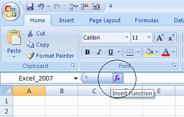
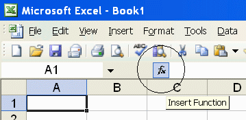
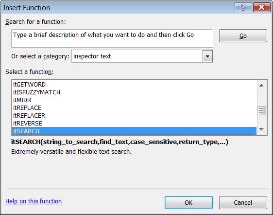
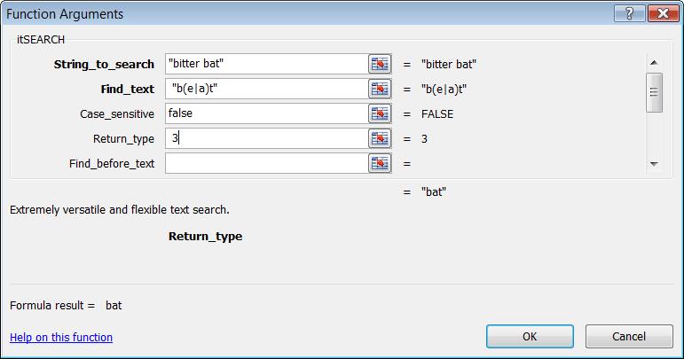
If you are using a paid edition of inspector text, you can use Excel's Insert Function dialog to insert xlPrecision functions more conveniently than typing them in directly:
|
Using Excel's Insert Function Dialog with the inspector text Free Edition Using Excel's Insert Function dialog with the inspector text Free Edition is not recommended because it calculates on every keystroke, causing the Free Edition dialog to appear many times more than usual. Although it is not recommended in the Free Edition, it is enabled in the Free Edition so that you can evaluate it. If you do use it in the Free Edition, you might want to use Notepad to copy/paste whole arguments instead of typing them in, to minimize the number of times the Free Edition dialog appears. |
The custom category "inspector text" is not always created successfully, especially with versions of Excel earlier than 2003. In that case, you can always find the inspector text functions in the "ALL" category.
For helpful tips on using xlPrecision, see:
For more detail on usage and syntax, please see:
For help on troubleshooting common problems, see: