PrecisionCalc
xl
Precision
Get Your Numbers Right
(When xlPrecision is installed, this tutorial
is also available from within Excel by choosing Tools | xlPrecision |
xlPrecision Help and Function Reference.)
Tutorial
(This is a detailed, in-depth tutorial. For a
quicker start, you may prefer to begin with the
Quick-Start Tutorial.)
The first step in learning to use
xlPrecision is to understand the limitations in Excel that xlPrecision solves.
This tutorial starts by walking you through those limitations, with simple
examples showing how xlPrecision solves them.
Then, in the
Using xlPrecision section, it goes into more
detail on getting the most from xlPrecision.
Excel Limitation #1:
15 Significant Digits
Excel's formulas often round their results.
-
Create a new workbook in Excel.
-
In cell A1, enter "67" (without quotes).
-
In cell A2, enter "89" (without quotes).
-
In cell A3, enter "=A1/A2" (without quotes).
-
Right-click cell A3 and choose Format Cells.
-
On the Number tab, in the Category listbox, select Number.
-
In the Decimal Places spinner, enter the maximum (30), and
click OK.
-
Widen column A as much as necessary to see the number.
-
Note that cell A3 shows:
0.752808988764045000000000000000
The correct answer would continue infinitely.
Excel returns only 15 significant digits.
(Significant digits is the quantity
of digits from the
left-most non-zero digit to the right-most non-zero digit, regardless of the
location of the decimal point.)
To see how xlPrecision solves that
limitation:
Excel Limitation #2:
Excel Automatically Rounds Your Numbers
When you enter a number in Excel, Excel often
permanently changes some of the digits to zero.
To see how xlPrecision solves that
limitation:
Excel Limitation #3:
Binary Conversion Errors
Even with
small numbers, Excel's formulas often return inexact results.
-
Create a new workbook in Excel.
-
In cell A1, enter "1000.8" (without
quotes).
-
In cell A2, enter "1000" (without quotes).
-
In cell A3, enter "=A1-A2" (without
quotes).
-
Note that cell A3 shows "0.8", which is
correct. But things are not as they seem. Excel is showing a slightly
different number than it is actually storing in cell A3. To see what number
Excel is actually storing in cell A3, continue with the following steps.
-
Right-click cell A3 and choose Format
Cells.
-
On the Number tab, in the Category listbox,
select Number.
-
In the Decimal places spinner, increase
decimal places to at least 15. Click OK.
-
Note that cell A3 now shows:
0.799999999999955 is the number Excel is
actually storing in A3, and that is the number that any formula referencing cell
A3 will be given to use. It's very close to 0.8. But with enough repetition, as
with summing a large range of numbers that each have a similar small inaccuracy,
the total discrepancy can become large.
To see how xlPrecision solves that
limitation:
-
Create a new workbook in Excel.
-
In cell A1, enter "9E+307" (without
quotes).
-
In cell A2, enter "1" (without quotes).
-
In cell A3, enter "=A1*A2" (without
quotes).
-
Note that cell A3 returns "9.00E+307",
indicating that the operation was successful. This shows that Excel is able to
work with numbers as large as 9E+307 (9 with 307 zeroes after it).
-
Now, change cell A2 from "1" to "10"
(without quotes).
-
Note that cell A3 now returns the error
value "#NUM!". This shows that Excel is unable to work with numbers as large
as 9E+308 (9 with 308 zeroes after it).
To see how xlPrecision solves that
limitation:
The same is true -- except worse! -- for numbers that are very close to zero:
-
In cell B1, enter "1E-307" (without
quotes).
-
In cell B2, enter "1" (without quotes).
-
In cell B3, enter "=B1/B2" (without
quotes).
-
Note that cell A3 returns "1.00E-307",
indicating that the operation was successful. This shows that Excel is able to
work with numbers as small as 1E-307 (a decimal point, then 306 zeroes, then a
1).
-
Now, change cell B2 from "1" to "10"
(without quotes).
-
Note that cell B3 now returns:
-
0.00E+00
-
This
indicates that as far as Excel is concerned, 1E-308 is actually equal
to zero! It would be far better for Excel to return the error value "#NUM!",
correctly indicating that it is unable to work with numbers that small.
-
Note that no matter how
large you make the number in cell B2, B3 continues to return "0.00E+00",
indicating that Excel still considers it equal to zero.
To see how xlPrecision solves that
limitation:
xlPrecision provides high precision in Excel by replacing
Excel's low precision arithmetic operators (+, - *, /, ^), comparison operators,
(>, >=, <, <=, =), and some of its worksheet functions (SUM, MEDIAN, RANK,
and many others), with custom worksheet functions, such as xlpADD,
xlpMULTIPLY, xlpISLESS, xlpMEDIAN, etc. For a complete list of xlPrecision
functions, see the
Function Reference.
Unfortunately, Excel does not allow changing the behavior
of its built-in operators and worksheet functions, so it is not possible for xlPrecision to apply high
precision to your existing worksheet formulas. Using xlPrecision requires
modifying your worksheet formulas by replacing Excel's built-in operators with
xlPrecision's custom worksheet functions. Of course, you only have to modify
those formulas from which you want high precision.
For example, to get high precision from this worksheet
formula:
=2/3
Change the formula to this:
=xlpDIVIDE(2,3)
Be sure to put a
comma (",")
between the 2 and the
3, not a slash ("/").
|
Depending on your world region and language, you might need to use a
different character than the comma.
Use whatever character you normally
use to separate arguments in Excel functions. In many locales, that
character is a semi-colon (;).
If you're not sure, go into Windows' Regional/Language Options Control Panel and
find your "List Separator" character. Use that character wherever xlPrecision
documentation shows a comma. This example shows that the list separator
character for French is the semi-colon:
|
The result should be as long as your edition of
xlPrecision allows, or the default length of 100 significant digits, whichever
is shorter. For example, if you are using the 25SD edition, the result
should be 25 significant digits long, like this:
0.6666666666666666666666667
xlPrecision results are returned as text that look like numbers,
not as values that Excel recognizes as numbers. This is because Excel would
immediately truncate the results to 15 significant digits if it recognized them as numbers.
You can use the results of xlPrecision formulas as the operands in other
xlPrecision formulas, but using them as operands in Excel's arithmetic functions will
truncate them to 15 significant digits.
If you have a complex formula with more than one
arithmetic operator or comparison operator, you may need to replace them all
with xlPrecision functions. For example, in this formula, Excel discards the
high precision returned by xlpDIVIDE when it evaluates the subtraction with
Excel's built-in operator, the minus sign:
=xlpDIVIDE(A1,B1)-C1
To maintain high precision in that example, replace the
minus sign with xlpSUBTRACT:
=xlpSUBTRACT(xlpDIVIDE(A1,B1),C1)
Avoid Long
Recalculations
When returning numbers with very high significant
digits, or with very large operands, xlPrecision can take a long time to
calculate. To prevent Excel from unnecessarily recalculating them, convert the
affected formulas to text by copying them and then Paste Special > Values. And
then be sure to save the workbook before closing it.
Specifying Quantity of
Significant Digits
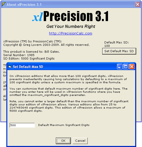
The number of significant digits xlPrecision provides depends on
the edition of xlPrecision you have. For example, the free edition provides 500
significant digits. Paid versions provide up to 32,767 significant digits. To
determine how many significant digits your edition of xlPrecision provides, go
to Excel's Tools menu and choose xlPrecision | About xlPrecision. One of the
lines on the About box that pops up starts with "SD Edition:" and indicates the
maximum number of significant digits your edition of xlPrecision provides.
Another way to determine how many significant digits your
edition of xlPrecision provides is to enter "=xlpSD()" in any cell (without
quotes, and xlpSD is not
case-sensitive). The number returned is the maximum number of significant digits
your edition of xlPrecision provides.
If you don't specify how many significant digits you want,
you'll get a maximum of 100, to prevent inadvertently starting long
calculations. You can customize that maximum in the About box:
For each xlPrecision function, you can specify any number of significant digits up to
32,767. For example, to get 1,000 significant digits, change the formula to
this:
=xlpDIVIDE(2,3,,,,,1000)
If you specify more significant digits than your
xlPrecision edition allows, then you'll get the maximum allowed by your edition.
Alternatively, you can specify fewer
significant digits to speed up calculation.
Depending on how many significant digits your
xlPrecision formula returns, the result may be too long to conveniently view. You can
view the full result by right-clicking the cell and choosing Format Cells |
Alignment | Wrap Text, and widening the column to the width of the screen. To
view the full result without changing column
widths or wrapping text, copy the cell and paste into Notepad or a word
processor.
Other Arithmetic
Operators
xlpADD(), xlpSUBTRACT(), xlpMULTIPLY(), xlpROOT(), and
xlpPOWER() all work
essentially the same way as xlpDIVIDE():
|
Change this: |
To this: |
|
=2+3 |
=xlpADD(2,3) |
|
=2-3 |
=xlpSUBTRACT(2,3) |
|
=2*3 |
=xlpMULTIPLY(2,3) |
|
=2/3 |
=xlpDIVIDE(2,3) |
|
=2^(1/3) |
=xlpROOT(2,3) |
|
=2^3 |
=xlpPOWER(2,3) |
The comparison operators are similar too:
|
Change this: |
To this: |
|
=2=3 |
=xlpISEQUAL(2,3) |
|
=2<>3 |
=xlpISNOTEQUAL(2,3) |
|
=2>3 |
=xlpISGREATER(2,3) |
|
=2>=3 |
=xlpISGREATEROREQUAL(2,3) |
|
=2<3 |
=xlpISLESS(2,3) |
|
=2<=3 |
=xlpISLESSOREQUAL(2,3) |
If any of the xlPrecision functions return "#VALUE!", make sure
you are separating the operands with a comma, not an arithmetic operator. For
example, if you enter "=xlpADD(A1+A2)" instead of
"=xlpADD(A1,A2)", it will return "#VALUE!".
For a complete list of xlPrecision functions,
along with detailed information on using them and examples, see the
Function Reference.
Long Operands
So far in this tutorial, the numbers in cells A1 and A2 are
entered in Excel as numbers. But if you use operands longer than 15 significant
digits, Excel will truncate them to 15 significant digits. For example:
-
In cell A1, change the number 67 to 12345678901234567890.
-
Right-click cell A1 and choose Format Cells.
-
On the Number tab, in the Category listbox, select Number.
-
In the Decimal Places spinner, enter the maximum (30), and
click OK.
-
Note that Excel truncated the number to 12345678901234500000
-- it didn't even round it correctly to 12345678901234600000.
xlPrecision is capable of using operands with up to 32,767
significant digits. But to prevent Excel from truncating them to 15 significant
digits, you'll need to enter them as text instead of as a number:
-
Right-click cell A1 and choose Format Cells,
-
On the Number tab, in the Category listbox, select Text
(not Number).
-
In cell A1, change the number 12345678901234500000 to
12345678901234567890.
Note that this time, Excel did not change it. That will work for
xlPrecision functions, but note that if you use it in a non-xlPrecision formula,
Excel will truncate the number again.
Alternatively, you can enter long operands
within the formula by enclosing them with double-quotes so that Excel treats
them as text rather than as numbers. For example, change the above formula to
this:
=xlpADD("123456789123456789123456789","123456789123456789123456789")
Formatting Negatives
By default, xlPrecision formats negative results with a leading
hyphen ("-"). On all editions except for the 25 SD edition, you can optionally
format negatives with parentheses ("()"):
-
In cell C4, change the formula "=xlpSUBTRACT(A1,A2)" to
"=xlpSUBTRACT(A1,A2,2)".
Note that the return value changes from "-86419753208641975320"
to "(86419753208641975320)".
The 3rd argument is "format_negative". The only valid values for
format_negative are 1 and 2. Entering 1 formats negatives with a leading hyphen.
Any values entered other than 1 or 2 are ignored, and negatives will be formatted with a
leading hyphen.
format_negative is ignored in the 25 SD edition, which always
formats negatives with a leading hyphen.
Negatives formatted with parentheses can be used as operands in
other xlPrecision formulas, as well as negatives formatted with leading hyphens.
Some xlPrecision functions use different
syntax than this for formatting negatives. See the
Function
Reference entries for each xlPrecision function.
Formatting Thousands Separators
By default, xlPrecision does not add thousands separators such
as the comma in "1,000". On all editions except for the 25 SD
edition, you can optionally add them:
-
In cell C4, change the formula "=xlpSUBTRACT(A1,A2,2)" to
"=xlpSUBTRACT(A1,A2,2,TRUE)".
Note that the return value changes from "(86419753208641975320)"
to "(86,419,753,208,641,975,320)".
The 4th argument is "format_thousands". format_thousands is
ignored in the 25 SD and 35 SD editions, which never return thousands
separators.
The thousands separator generated by format_thousands is
internationalized. This means that the local thousands separator will be used --
for example, a comma in the USA, a period in Germany, and a space in France.
Note, the decimal symbol is also internationalized -- for example, a period in
the USA, a comma in Germany and France.
Results formatted with thousands separators can still be used as operands in
other xlPrecision formulas.
Some xlPrecision functions use different
syntax than this for formatting thousands separators. See the
Function
Reference entries for each xlPrecision function.
Formatting Currency
On all editions except for the 25 SD edition,
results can optionally be formatted with the local currency symbol (for
example, "$" in the USA):
-
In cell C4, change the formula "=xlpSUBTRACT(A1,A2,2,TRUE)" to
"=xlpSUBTRACT(A1,A2,2,TRUE,TRUE)".
Note that the return value changes from "(86,419,753,208,641,975,320)"
to "($86,419,753,208,641,975,320)".
The 5th argument is "format_currency". format_currency is
ignored in the 25 SD edition.
Results formatted with the local currency symbol can still be
used as operands in other xlPrecision formulas.
Some xlPrecision functions use different
syntax than this for formatting currency. See the
Function
Reference entries for each xlPrecision function.
Formatting in Exponential
Notation
On all editions except for the 25 SD edition,
results can optionally be formatted in exponential notation:
-
In cell C4, change the formula "=xlpSUBTRACT(A1,A2,2,TRUE,TRUE)" to
"=xlpSUBTRACT(A1,A2,2,TRUE,TRUE,TRUE)".
Note that the return value changes from "($86,419,753,208,641,975,320)"
to "($8.641975320864197532E+19)".
The 6th argument is "exponential_notation".
exponential_notation is
ignored in the 25 SD edition.
Results formatted with exponential notation can still be
used as operands in other xlPrecision formulas.
Some xlPrecision functions use different
syntax than this for formatting exponential notation. See the
Function
Reference entries for each xlPrecision function.
Formatting Decimal
Place
On the 5,000 SD edition and higher,
and on the Free Edition, results can optionally be formatted to any
decimal place you specify.
-
In cell C4, change the formula to
"=xlpSUBTRACT(A1,A2,,,,,,,3)".
Note that the return value changes
to "86,419,753,208,641,975,320.000".
The 9th argument is "format_decimal_place".
format_decimal_place is
ignored in the 25 SD and 1,500 SD editions.
format_decimal_place was added in version
3.1, and currently applies only to the
arithmetic operator functions, and to xlpFORMAT.
Getting Faster Calculations
If you don't specify how many significant
digits to return, you'll get 100, or less if your edition of xlPrecision only
allows fewer than that. You can get faster calculations by specifying a lower
number of significant digits. For example, this formula specifies 50 significant
digits:
=xlpDIVIDE(2,3,,,,,50)
Displaying &
Printing Results Longer Than 1,024 Characters
Microsoft Excel 97 and later allows up to 32,767
text characters in a cell, and Excel 2007 and later can display and print all of them.
However, Excel normally displays only the
first 1,024 characters in a cell. To view an xlPrecision return value longer
than 1,024 characters, turn on "Wrap Text" for the cell:
- To turn on "Wrap Text" for the cell,
right-click the cell and choose Format Cells. Then Select the Alignment tab,
and turn on Wrap Text.
After turning on Wrap Text, you'll probably also need to
widen the column and make the row height taller, and maybe make the font size
smaller.
However, although that will display more than
1,024 characters, in Excel versions earlier than 2007 it won't display 32,767
characters. The exact number of characters it will display varies depending on
your configuration. To view all 32,767 characters, you can do any of the
following:
-
Copy the cell, and Paste Special | Values to
another cell. Then, with the new cell selected, look in the formula bar. The
formula bar displays the entire result (up to 32,767 characters), though you may
need to scroll down within the formula bar to see it all.
-
Copy the cell and paste into Notepad or a
word processor.
-
Save the file as a text file type (Save As
| Save as type = "text (tab delimited)"), and view the text file in Notepad or a
Word processor.
-
Using the Text Box tool on Excel's Drawing
toolbar, draw a textbox on the worksheet. Select the cell and Copy | Paste
Special | Values to another cell. With the new cell selected, click in the
formula bar and select the entire contents. Copy the contents, and paste into
the textbox.
Also, in Excel 2007 and later, you can view
up to 8,192 characters in the formula bar by selecting the formula in the
formula bar, and pressing F9 (but don't press Enter!). When done, be sure to
press Escape to bring back the formula. If you inadvertently press Enter, try
Undo (Ctrl + z) to bring back the formula.
To display and print all 32,767 characters in
a cell in Excel 2007, you'll need to make the font size very tiny, in addition
to maximizing the column width and row height. In some cases you may prefer some
of the above workarounds even in Excel 2007.
Although Excel normally displays and prints
only the first 1,024 characters in the cell, it makes all the characters (up to
32,767 characters) available to formulas in other cells, including xlPrecision
formulas. The display of only 1,024
characters does not indicate any loss of precision in xlPrecision formulas.
32,767 SD Edition: Special Considerations
The 32,767 SD edition is only able to return 32,767 significant
digits when the result is a positive integer not formatted with either thousands
separators or currency symbols. This is because Excel only allows a maximum of
32,767 characters in a cell. If one of those characters is a decimal, then only
32,766 characters are left over for digits. The same is true of currency symbols
and negative formatting. If the number is smaller than 1, then zeroes between
the decimal and the first significant digit will also reduce the available
number of significant digits. And of course, thousands separators can reduce it
by up to 25%.
In all cases, the 32,767 SD edition will give you as many
significant digits as possible with the formatting you have chosen.
If the return value is so large that it has more than 32,767
characters to the left of the decimal, then xlPrecision is of course unable to
return a correct value and instead returns "#VALUE!". Note, that's a
vastly larger
number than Excel can return without xlPrecision. Excel itself can only return
or recognize a number with a maximum of 308 digits to the left of the decimal.
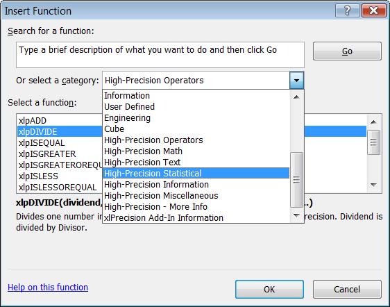
Insert Function
Dialog
If you are using the 1,500 SD or higher edition, or the
Free Edition, of xlPrecision, you can use Excel's Insert Function dialog to
insert xlPrecision functions more conveniently than typing them in directly:
- Select the worksheet cell where you want the
xlPrecision formula.
- Click the little "fx"
to the left of Excel's formula bar. Or, click Formulas | Insert Function (in
Excel 2003 and earlier, choose Insert | Function). The Insert
Function dialog should appear.
- In the Insert Function dialog, bring down the Category
dropdown, and select any of the High-Precision categories at the bottom of the
list. The function list should show the xlPrecision functions in that
category.
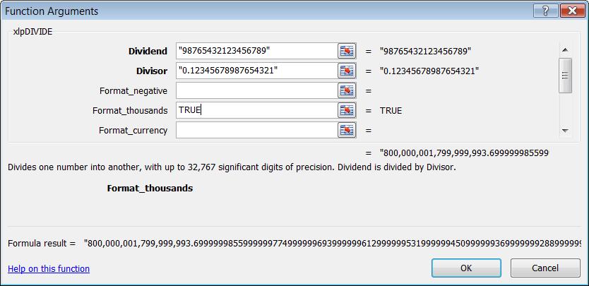
- Select a function and click OK. The Function Arguments
dialog should appear for that function.
- For each of the argument fields, you can either type
the argument in directly, or click the little square to the right of it,
select a cell where you've put the desired argument. When you're done, click
OK.
- If at any time you want to modify an
existing xlPrecision
formula, simply select that cell and click the little "fx"
to the left of Excel's formula bar or choose Insert | Function. Instead of the
Insert Function dialog, you'll then get the Function Arguments dialog, already
filled out with the arguments you've already entered. Then, simply change them
as desired and click OK.
Using the Insert Function dialog with xlPrecision
functions requires the 1,500 SD or higher edition, or the Free Edition, of
xlPrecision. Not recommended with the Free Edition as it causes the Free Edition
dialog to appear multiple times.
|
Using
Excel's Insert Function Dialog with the xlPrecision Free Edition
Using Excel's Insert Function dialog with the
xlPrecision Free Edition is not recommended
because it calculates on every keystroke, causing the Free Edition
dialog to appear many times more than usual.
Although it is not recommended in the Free
Edition, it is enabled in the Free Edition so that you can evaluate it.
If you do use it in the Free Edition, you might
want to use Notepad to copy/paste whole arguments instead of typing them
in, to minimize the number of times the Free Edition dialog appears. |
Using Excel's Insert Function Wizard can be slow because
Excel recalculates the function every time a digit or character is entered in
the Wizard. To speed up that process, enter "0" for all numeric operands (such
as num and rt for xlpROOT), so that the function does not take long to
calculate. Then, when done with the Wizard, manually change the numeric operands
to the desired numbers directly in the worksheet. Alternatively, you could use
Notepad to copy/paste whole arguments instead of typing them in.
Factorials
An interesting way to compare xlPrecision
with Excel is to look at how they calculate factorials. A factorial is
the number resulting from multiplying a whole number by every whole number
between itself and 1, inclusive. For example, the factorial of 5 is:
1
x 2 x 3 x 4 x 5 = 120
Factorials are symbolized with an exclamation
point ("!"). For example, the factorial of 5 is represented as "5!". An example
of how factorials are used is to determine the total possible number of ways a
given number of items can be arranged in a row. For example, the factorial of a
standard deck of playing cards is 52!.
Without xlPrecision, Excel can calculate
factorials up to 170!. But it can only calculate factorials at full precision
up to 20! -- after that, Excel rounds them to the first 15 digits. xlPrecision
can calculate factorials up to 9,273! -- all at full precision.
To see it for yourself:
-
Create a new workbook in Excel.
-
In cell A1, enter "=ROW()" (without quotes).
-
Copy cell A1 down through A200.
-
In cells B1 and C1, enter "1" (without
quotes).
-
In cell B2, enter "=xlpMULTIPLY(B1,A2)"
(without quotes).
-
In cell C2, enter "=C1*A2" (without quotes).
-
Copy cells B2 and C2 down to B200 and C200.
(But note, if you're using the Free Edition, you'll need to click OK once per
row, so you might want to start out with fewer rows.)
-
Select column C, and choose Format | Cells |
Number tab. In the Category dropdown listbox, select Number. In the Decimal
Places spinner, select 0.
-
Widen columns B and C so that you can see as
much of them both together as possible.
-
Note that on rows 1 - 20, Excel (column C)
and xlPrecision (column B) are identical.
-
Note that cells B21 and C21 are different. In
C21, excel has rounded it down. That's because 21! has 16 non-zero digits, and
Excel can only give you the first 15 of them. xlPrecision, in cell B21, gives
you all 16 non-zero digits.
-
Note that at row 171, Excel (column C) starts
returning "#NUM!". That's because Excel can't recognize a number that large.
-
xlPrecision can return factorials down
through row 9,273, though the precision depends on the xlPrecision edition. The
32,767 SD edition can return 9,273! at full precision, and the 1,500 SD edition
can return 693! at full precision. The 35 SD and 25 SD editions can return 36!
and 29! respectively at full precision, which may not sound like much but are
still better than Excel's 20! at full precision.
-
Getting back to the deck of playing cards
(52!), Excel (cell C52), rounding 52! to 15 significant digits, returns:
80,658,175,170,943,900,000,000,000,000,000,000,000,000,000,000,000,000,000,000,000,000,000
80,658,175,170,943,878,571,660,636,856,403,766,975,289,505,440,883,277,824,000,000,000,000
(That number is precisely correct -- the final 12 zeroes are not
due to rounding.)
21,428,339,363,143,596,233,024,710,494,559,116,722,176,000,000,000,000
Data Control & Analysis Features
xlPrecision offers many additional features that take you
beyond Excel's capabilities in other ways. See
Data Control & Analysis
Features.
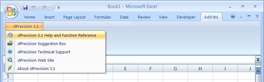
Online Help
Find xlPrecision's online help by choosing Add-Ins
> xlPrecision 3.1
> xlPrecision 3.1 Help and
Function Reference:
In Excel 2003 and earlier, xlPrecision's online help is in Tools
> xlPrecision 3.1
> xlPrecision 3.1 Help and
Function Reference:
For helpful tips on using xlPrecision, see:
Tips
For more detail on usage and syntax, please see:
Function Reference
For help on troubleshooting common problems, see:
Troubleshooting F.A.Q.
xlPrecision
Home Page
PrecisionCalc Home Page